Sol Gets a numbered sunspot

Near-Live image of the sun in 304 angstrom as seen by NASA’s SDO.

It has been a surprise in the last 12 months to see a numbered sunspot on the face of Sol, but we have one today in NOAA Active Region 2575 (Catania sunspot group 28). The sunspot is stable but inactive. This image is for that part of teh spectrum centred on 304 Angstroms where photons are emitted by Helium 2 at around 50,000C, in the chromosphere and the transition region. Solar activity is expected to remain low with a low probability of flares or mass ejections.

In the past 24 hours the solar wind speed remained slightly enhanced under the influence of a negative polarity coronal hole and increased from around 400 to 520 km/s. The total interplanetary magnetic field strength was in the range of within 5-8nT in the beginning of the period and has decreased to below 3nT at 12 UTC today. The Bz component was mostly negative with a minimum value of -7 nT. The solar wind conditions are expected to remain enhanced over the next 24 hours.

Sunspots on the face of our star remain few in number as we are in the middle of the solar minimum. Solar Cycle 25 will be the 25th Solar Cycle since 1755. Solar cycles are marked by a reversal in magnetic polarity, with the first convincingly reversed sunspots of SC 25 occuring in November 2019. SC 25 solar maximum should occur between 2023 and 2026 with 2031 seeing the end of the cycle. The strength of SC 25 is debated with predictions of 30-50% of SC24 to somewhat stronger than SC24.

Arctic Sea Ice Extent 25/01/2020

January 27, 2020

Mapped Arctic sea ice extent (SIE) on 25/01/2020 was 14.11 million km2 which is 420,000 km2 or 2.9% less than the 2008-2018 median.  This is largest sea ice extent on this day since 2014. The current sea ice accumulation rate is 65,000 km2/day, the fifth highest since 1979.

Figure 1 MASIE Arctic Sea Ice Extent and SIE Median for the period 1981-2010

Figure 2 Arctic Sea Ice Extent (MASIE Database – see above image) for the month of January for the period 2000-2020 with the 1988-2018 median

The extent of Arctic sea ice varies from summer to winter. The sea ice extent shown here relies on data from the Multisensor Snow and Ice Mapping System (IMS) that runs at the National Ice Center. The IMS product uses several satellite data sources including passive microwave, but it is also based on visual analysis and other data sources and undergoes a form of manual data fusion. The data reported here has a 1 km resolution and was sourced from the National Snow and Ice Data Center

Arctic Sea Ice Extent 16/01/2020

January 17, 2020

Mapped Arctic sea ice extent (SIE) on 15/1/2020  was 13.57 million km2 which is 560,000 km2 or 4% less than the 2008-2018 median.  This is largest sea ice extent on this day since 2015.

MASIE Arctic Sea Ice Extent and SIE Median for the period 1981-2010
Arctic Sea Ice Extent (MASIE Database – see above image) for the month of January for the period 2000-2020 with the 1988-2018 median

The extent of Arctic sea ice varies from summer to winter. The sea ice extent shown here relies on data from the Multisensor Snow and Ice Mapping System (IMS) that runs at the National Ice Center. The IMS product uses several satellite data sources including passive microwave, but it is also based on visual analysis and other data sources and undergoes a form of manual data fusion. The data reported here has a 1 km resolution and was sourced from the National Snow and Ice Data Center

Arctic Sea Ice Accumulation in 2019 Approaches Record High

Daily Rate of Arctic Sea Ice Accumulation in 2019 Approaches Record High

The well known reduction in Arctic Sea Ice extent during the summer months continued during 2019. This trend has been recorded since the beginning of the satellite instrumental record. The minimum ice extent has fallen from 6.9 million km2 in 1979 to 4 million km2 in 2019 while the maximum ice extent has fallen from 16.6 million km2 to 14.9 million km2 in 2019.

The median ice extent shows a consistent linear trend from 12.8 million km2 in 1979 to 11 million km2 in 2019.

Figure 1 Minimum, Maximum and Media of Arctic sea ice for the period 1979 through 2019

The average daily rate of melting from April through August has increased from 54,000 km2 per day in 1979 to peak in 2011 at 74,000 km2 per day.

Interestingly the daily rate rate of sea ice accumulation in the period October through December has increased from 67,000km2 in 1979 to peak at 95,000km2 in 2012. The current daily rate of accumulation in 2019-2020 is again approaching the highest levels in the instrumental record. Difficult to see anything other than natural processes in this record given its limited duration. Historic records however suggest that the low summer ice extent recorded of recent time was as common in the early 20th century.

Figure 2 Rate of melting (Red) and Accumulation (Blue) of Arctic Sea Ice during the period 1979 through 2019

The sea ice extent data discussed here relies on data from the Multisensor Snow and Ice Mapping System (IMS) that runs at the National Ice Center. The IMS product uses several satellite data sources including passive microwave, but it is also based on visual analysis and other data sources and undergoes a form of manual data fusion. The data reported here was sourced from the National Snow and Ice Data Center.

ARCTIC SEA ICE EXTENT 11/01/2020

January 11, 2020

Mapped Arctic sea ice extent (SIE) on this date was 13.34 million km2 which is 560,000 km2  or 4% less than the 2008-2018 median.  This is largest sea ice extent on this day since 2016

MASIE Arctic Sea Ice Extent and SIE Median for the period 1981-2010
Arctic Sea Ice Extent (MASIE Database – see above image) for the month of January for the period 2000-2020 with the 1988-2018 median

The extent of Arctic sea ice varies from summer to winter. The sea ice extent shown here relies on data from the Multisensor Snow and Ice Mapping System (IMS) that runs at the National Ice Center. The IMS product uses several satellite data sources including passive microwave, but it is also based on visual analysis and other data sources and undergoes a form of manual data fusion. The data reported here has a 1 km resolution and was sourced from the National Snow and Ice Data Center

Aussie Weather and the Indian Ocean Dipole

Of recent times all the reporting on Australia has been little more than dire warnings and catastrophic coverage. There is however some positive news on the horizon.

Australia’s climate is determined in large part by three major atmospheric circulatory systems, the Indian Ocean Dipole (IOD) the El Nino – Southern Oscillation (ENSO) and the Southern Annular Mode (SAM) illustrated in the following diagram.

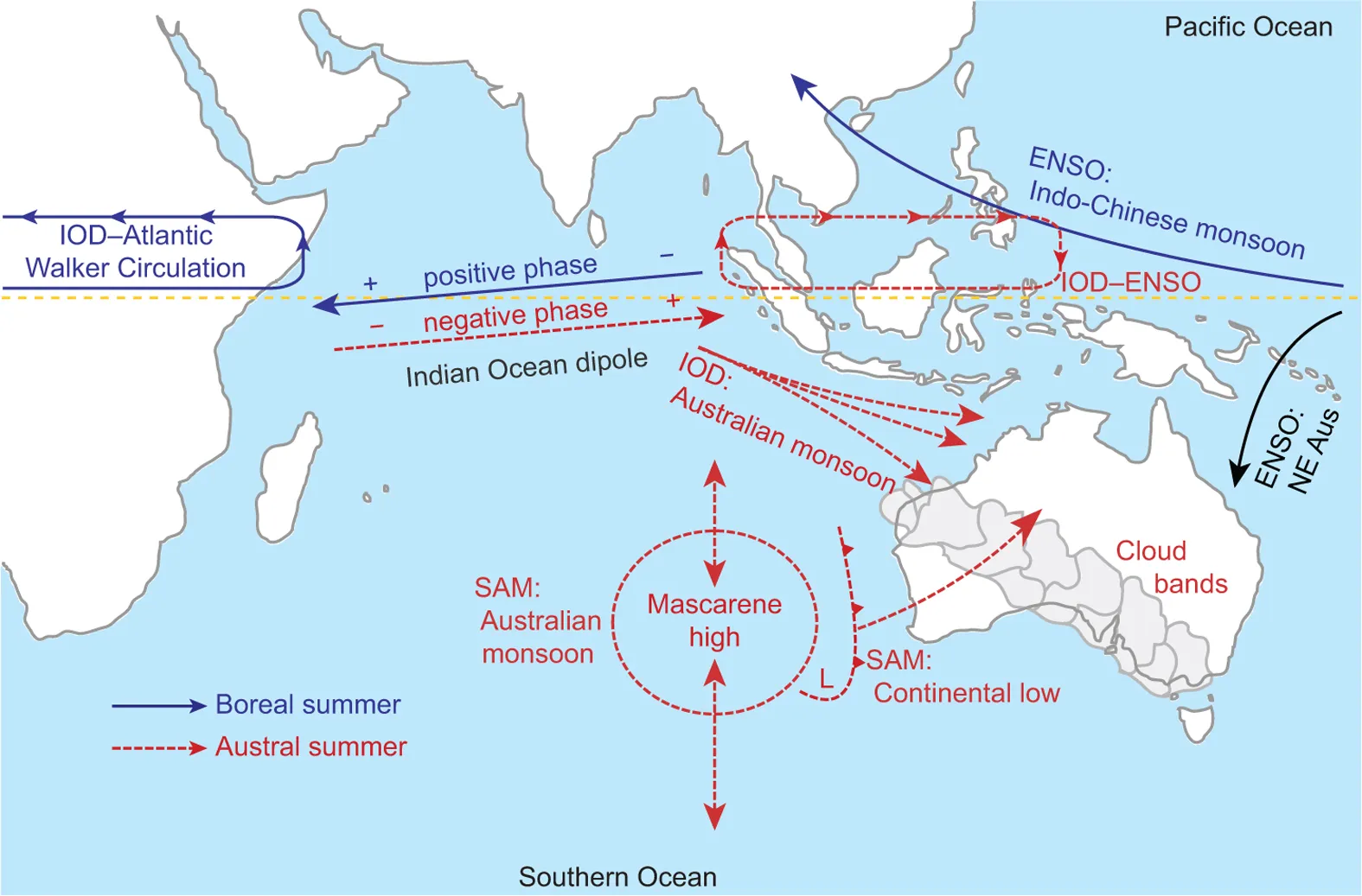
Figure 1 Coupled ocean–climate system in the Indian Ocean region during boreal (solid blue lines) and austral (dashed red lines) summer. Credit Cleverly, J., et al 2016

Indian Ocean Dipole

Within the northern Indian Ocean there is a major atmospheric circulation system which determines much of the weather patterns that impact Australia. A regular oscillation of sea surface temperatures (SST) occurs in the Indian Ocean and is known as the Indian Ocean Dipole (IOD) and is comparable to the better-known ENSO of the Pacific Ocean. The IOD results in SSTs becoming alternately warmer in the west and cooler in the east along the Western Australian coastline (warmer phase) and then colder in the west and warmer in the east (the negative phase).

A positive phase sees greater-than-average sea-surface temperatures and greater precipitation in the western Indian Ocean region, with a corresponding cooling of waters in the eastern Indian Ocean—which tends to cause droughts in adjacent land areas of Indonesia and Australia. The negative phase of the IOD brings about the opposite conditions, with warmer water and greater precipitation in the eastern Indian Ocean, and cooler and drier conditions in the west. This results in increased monsoonal activity in the NE Indian Ocean and increased injection of moisture into the Australian atmospheric system.

The strong IOD experienced during the first half of 2019 and the neutral ENSO and negative SAM created the very dry conditions which results in record low precipitation in Australia for 2019. Since October the IOD has fallen rapidly and while the BoM suggests that it will remain neutral it is equally likely that it will become strongly negative resulting in increased injection of moistures into the Australian atmospheric system later in 2020.

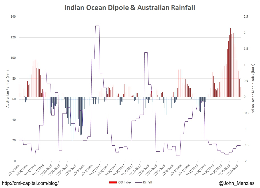
Figure 2 Australian Rainfall and Indian Ocean Dipole Index (Data after BoM)

El Nino – Southern Oscillation

El Niño and La Niña are the warm and cool phases of a recurring climate pattern across the tropical Pacific—the El Niño-Southern Oscillation, (ENSO).

The pattern can shift back and forth irregularly every two to seven years, and each phase triggers predictable disruptions of temperature, precipitation, and winds. El Niño describes a particular phase of the ENSO climate cycle when sea surface temperatures in the central and eastern tropical Pacific Ocean become substantially warmer than average, and this causes a shift in atmospheric circulation. Typically, the equatorial trade winds blow from east to west across the Pacific Ocean. El Niño events are associated with a weakening, or even reversal, of the prevailing trade winds. Warming of ocean temperatures in the central and eastern Pacific causes this area to become more favourable for tropical rainfall and cloud development. As a result, the heavy rainfall that usually occurs to the north of Australia moves to the central and eastern parts of the Pacific basin producing drought conditions in Australia.

In the Pacific Ocean, although indicators of the El Niño–Southern Oscillation (ENSO) are neutral, the tropical ocean near and to the west of the Date Line remains warmer than average, potentially drawing some moisture away from Australia.

Southern Annular Mode

The Southern Annular Mode, or SAM, is a climate driver that can influence rainfall and temperature in Australia. The SAM refers to the (non-seasonal) north-south movement of the strong westerly winds that blow almost continuously in the mid- to high-latitudes of the southern hemisphere as an annulus around Antarctica. This belt of westerly winds is also associated with storms and cold fronts that move from west to east, bringing rainfall to southern Australia.

The SAM has three phases: neutral, positive and negative. Each positive or negative SAM event tends to last for around one to two weeks, though longer periods may also occur. The time frame between positive and negative events is quite random, but typically in the range of a week to a few months. During summer a positive SAM can result in increased rainfall in SE Australia while during winter a positive SAM will see lower rainfall in Southern Australia and a negative SAM will allow more cold fronts to impact southern and SW Australia. In recent months SAM has moved from negative to neutral.

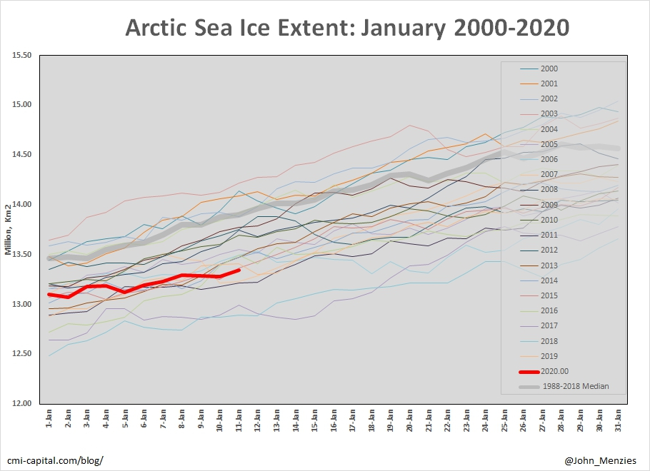
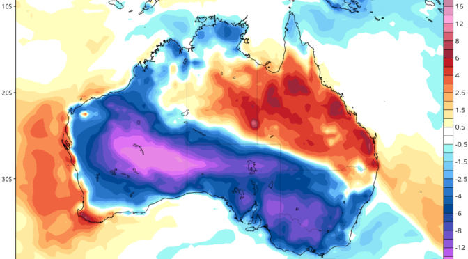
Forecast for January

The Global Ensemble Prediction System (GEPS) is an ensemble product of the Global Environmental Multiscale Model, an integrated data assimilation and forecasting system that runs for 16 days (384 hours). The graphics below shows the GEPS 2m temperature and precipitation output from 12th to the 28th January at 6-hour time intervals.

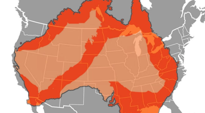
The GEPS model suggests that large areas of southern Australia should experience temperatures consistently below the seasonal average (by as much as 20C) but with little significant precipitation. Some rain in the WA wheat belt and subsequently in eastern states is predicted as tropical cyclone, Claudia, develops into a rain depression off the coast. Precipitation typical for northern Australia in summer is noted.

Figure 2 GEPS 2m Temperature Model for Australia through January 28th

Figure GEPS Precipitation model for Australia through January 28th

Will Britain’s’ Exclusive Offshore Economic Zone be Returned to its Rightful Owners?

The United Kingdom has a land area of 242,500 km2. In addition to this, is has a much larger, 731,300km2 Exclusive Economic Zone (EEZ), to which it surrendered rights to the European Union upon joining that body.

The map below shows the considerable and dominant EEZ in Europe in red.

An exclusive economic zone (EEZ) is a sea zone prescribed by the 1982 United Nations Convention on the Law of the Sea over which a state has special rights regarding the exploration and use of marine resources, including energy production from water and wind. It stretches from the baseline out to 200 nautical miles (nmi) from its coast. The term does not include either the territorial sea or the continental shelf beyond the 200 nmi limit. The difference between the territorial sea and the exclusive economic zone is that the first confers full sovereignty over the waters, whereas the second is merely a “sovereign right” which refers to the coastal state’s rights below the surface of the sea.

As an independent coastal state under the UN Convention on the Law of the Sea, the United Kingdom will be required to manage the living resources and fishing activities within its Exclusive Economic Zone in a sustainable way. Consequently, it will be for the UK Government, and the Devolved Administrations, to develop and implement a domestic fisheries policy after withdrawal from the EU. In declaring an Exclusive Economic Zone independent from EU waters, the UK would be able to control the access that foreign vessels have to fishing in UK waters. It will be for the Government of the day to decide whether the principle of equal access should be preserved, and the extent to which foreign vessels should be granted access to fishing in the UK EEZ.

The issues are relatively complex as several continental European countries have economic interests in the fisheries that lie within Britain’s EEZ. Britain could elect to continue to allow access or could deny it which could see a return to the Cod Wars of last century when there was frequent conflict between British and Icelandic fishermen in the Atlantic.

The Cod Wars were a national humiliation in the period 1958-1976, will it happen again?

Alternatively and more likely, as an interim move Britain could modify the quota system under the Common Fisheries Policy to the greater benefit of British coastal communities.

Reversion of its rights following BREXIT will be a hard fought battle but one worth fighting as it will allow for rapid expansion of the domestic fishing industry, decimated by Brussels and revitalize coastal communities which have supported BREXIT.

ARCTIC SEA ICE EXTENT 7/01/2020

January 7, 2020

Mapped Arctic sea ice extent (SIE) on this date was 13.23 million km2 which is 470,000 km2  or 3% less than the 2008-2018 median.  This is largest sea ice extent on this day since 2014

MASIE Arctic Sea Ice Extent and SIE Median for the period 1981-2010
Arctic Sea Ice Extent (MASIE Database – see above image) for the month of January for the period 2000-2020 with the 1988-2018 median

The extent of Arctic sea ice varies from summer to winter. The sea ice extent shown here relies on data from the Multisensor Snow and Ice Mapping System (IMS) that runs at the National Ice Center. The IMS product uses several satellite data sources including passive microwave, but it is also based on visual analysis and other data sources and undergoes a form of manual data fusion. The data reported here has a 1 km resolution and was sourced from the National Snow and Ice Data Center

Australia Bushfires – When Journalism Lies

Extent of Eastern Australian bushfires as of 7/01/2020. Data from the Victorian and New South Wales Rural Fires organisations.

The bushfire drama in Australia has subsided for the moment so now is a good time to take stock. As of 7/1/2020, the bushfires have devastated an area in Victoria and New South Wales of 49,600 km2.  In eastern Victoria the total burnt area was 12,100 km2 while in New South Wales it was 37,500km2.  

Various media outlets have been reporting more than 100,000 km2 was impacted by bushfires in eastern Australia which is a significant and entirely unnecessary exaggeration.

The prize for journalistic deceit however goes to Matt Zarrel of US, ABC News where he breathlessly shows a map of Australia superimposed on the USA.  The extent of the fires shown on this map (see below) totals 3.6 million km2, slightly less than half of the surface area of the continent or 60 times larger than the reality.  I doubt that anyone can be surprised.

ABC news was so embarrassed by the gross exaggeration they  removed the graphic.  

While the Australian Bushfires in 2019-2020 have been widespread it is worth noting that such events in Australia are not uncommon  as can be seen for the tabulation below for the state of Victoria.  The fires of 1939 covered 35,000 km2, a significant multiple to the 2019-2020 fires which were more comparable in scale to the 2003 and 2007 events.

ARCTIC SEA ICE EXTENT 4/01/2020

January 4, 2020

Mapped Arctic sea ice extent (SIE) on this date was 13.12 million km2 which is 430,000 km2  or 3% less than the 2008-2018 median.  This is largest sea ice extent on this day since 2014 and the 12th highest since 2000.    We predict maximum SIE of 15 million km2 to be reached in early April 2020.

MASIE Arctic Sea Ice Extent and SIE Median for the period 1981-2010

Arctic Sea Ice Extent (MASIE Database – see above image) for the month of January for the period 2000-2020 with the 1988-2018 median

The extent of Arctic sea ice varies from summer to winter. The sea ice extent shown here relies on data from the Multisensor Snow and Ice Mapping System (IMS) that runs at the National Ice Center. The IMS product uses several satellite data sources including passive microwave, but it is also based on visual analysis and other data sources and undergoes a form of manual data fusion. The data reported here has a 1 km resolution and was sourced from the National Snow and Ice Data Center